Minimum spanning trees#
Using the distances and a network, you can generate a minimum spanning tree. This can be useful when a neigbour joining tree is difficult to produce, for example if the dataset is very large, and in some cases has uses in tracing spread (take care with this interpretation, direction is not usually obvious).
There are three different ways to make MSTs, depending on how much data you have. Roughly:
‘Small’: Up to \(\sim 10^3\) samples.
‘Medium’: Up to \(\sim 10^5\) samples.
‘Large’: Over \(10^5\) samples.
In each mode, you can get as output:
A plot of the MST as a graph layout, optionally coloured by strain.
A plot of the MST as a graph layout, highlighting edge betweenness and node degree.
The graph as a graphml file, to view in Cytoscape.
The MST formatted as a newick file, to view in a tree viewer of your choice.
With small data#
For a small dataset it’s feasible to find the MST from your (dense) distance matrix.
In this case you can use Creating visualisations with the --tree option:
use --tree both to make both a MST and NJ tree, or --tree mst to just make
the MST:
poppunk_visualise --ref-db listeria --tree both --microreact --output dense_mst_viz

Graph-tools OpenMP parallelisation enabled: with 1 threads
PopPUNK: visualise
Loading BGMM 2D Gaussian model
Completed model loading
Generating MST from dense distances (may be slow)
Starting calculation of minimum-spanning tree
Completed calculation of minimum-spanning tree
Drawing MST
Building phylogeny
Writing microreact output
Parsed data, now writing to CSV
Running t-SNE

Done
Note the warning about using dense distances. If you are waiting a long time at this point, or running into memory issues, considering using one of the approaches below.
Note
The default in this modeis to use core distances, but you can use accessory or Euclidean
core-accessory distances by modifying --mst-distances.
This will produce a file listeria_MST.nwk which can be loaded into Microreact,
Grapetree or Phandango (or other tree viewing programs). If you run with --cytoscape,
the .graphml file of the MST will be saved instead.
You will also get two visualisations of a force-directed graph layout:
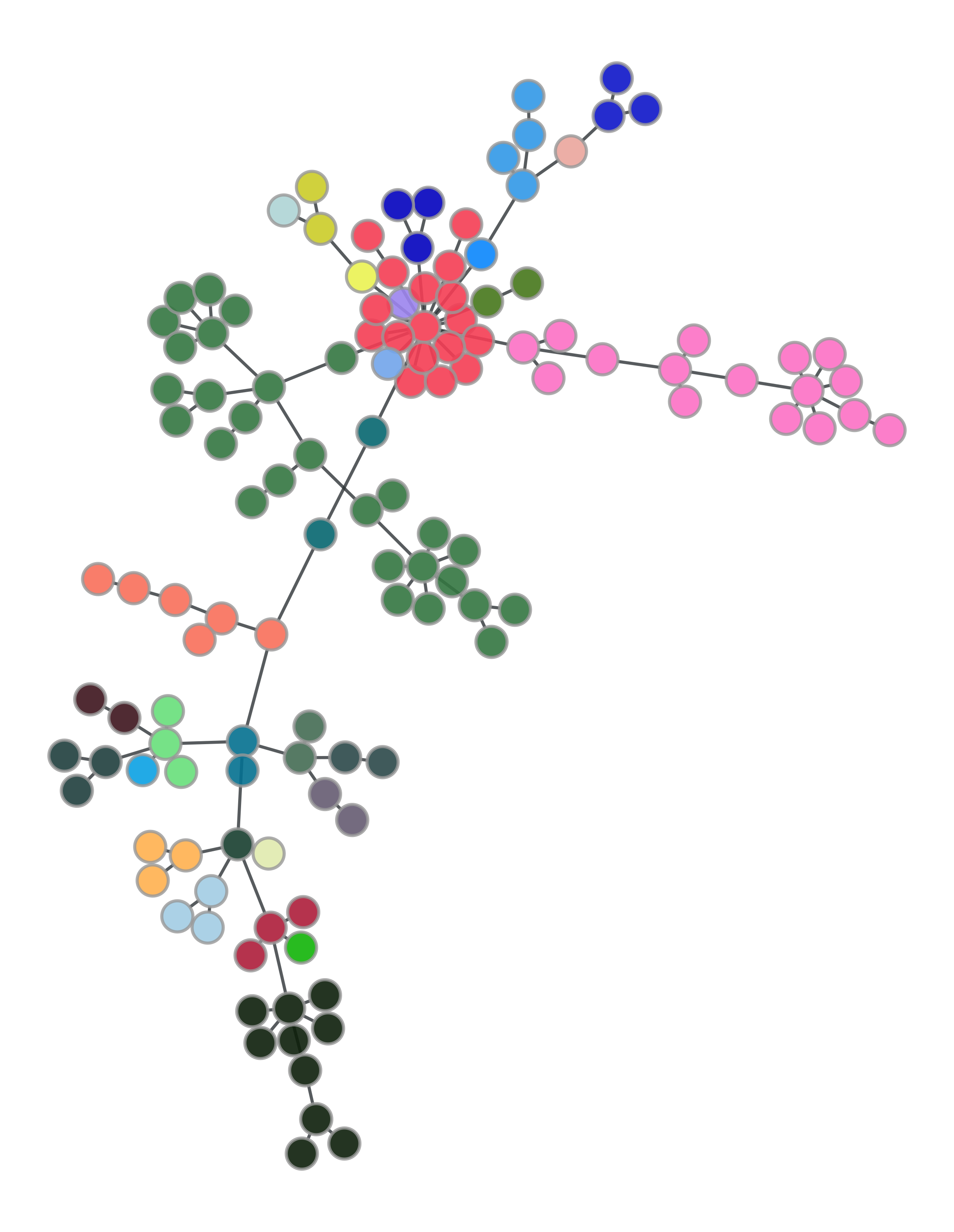
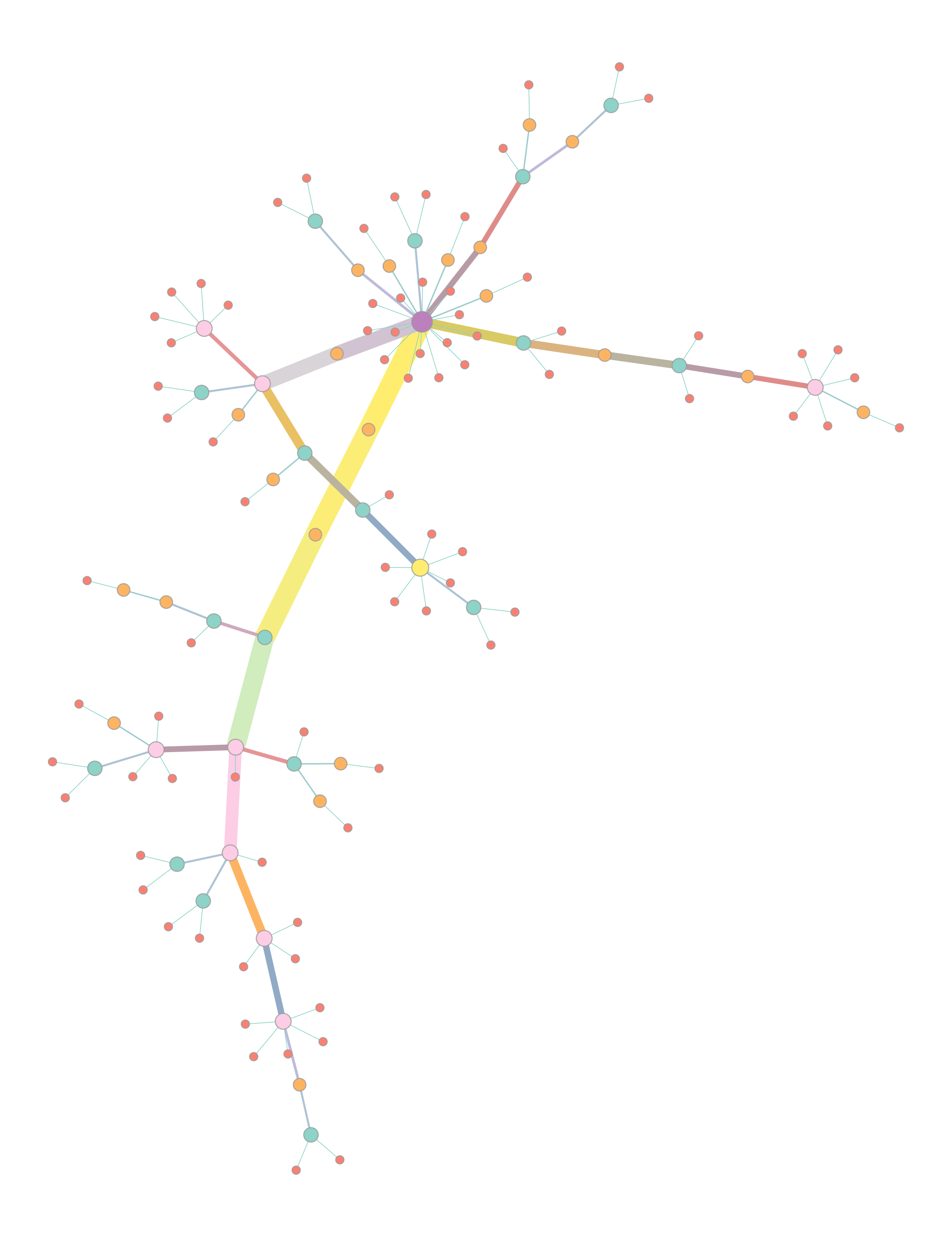
The left plot colours nodes (samples) by their strain, with the colour selected at random. The right plot colours and sizes nodes by degree, and edges colour and width is set by their betweenness.
With medium data#
As the number of edges in a dense network will grow as \(O(N^2)\), you will likely find that as sample numbers grow creating these visualisations becomes prohibitive in terms of both memory and CPU time required. To get around this, you can first sparisfy your distance matrix before computing the MST. The lineage mode does exactly this: keeping only a specified number of nearest neighbours for each sample.
Therefore, there are two steps to this process:
Fit a lineage model to your data, using a high rank.
Use
poppunk_mstto make the MST from the sparse matrix saved by this mode.
As an example, two commands might be:
poppunk --fit-model lineage --ref-db listeria_all --ranks 50 --threads 4 --output sparse_mst

poppunk_visualise --ref-db listeria --tree both --microreact  \
--rank-fit sparse_mst/sparse_mst_rank50_fit.npz --output sparse_mst_viz --threads 4
Ideally you should pick a rank which is large enough to join all of the components together. If you don’t, components will be artificially connected by nodes with the largest degree, at the largest included distance. Look for components to be one:
Network for rank 100
Network summary:
        Components      1
        Density 0.3252
        Transitivity    0.5740
        Score   0.3873
This will produce a <name>_rank100_fit.npz file, which is the sparse matrix to load. You will
also need your dense distances, but only the .pkl file is loaded to label the samples.
--previous-clustering is optional, and points to any .csv output from PopPUNK.
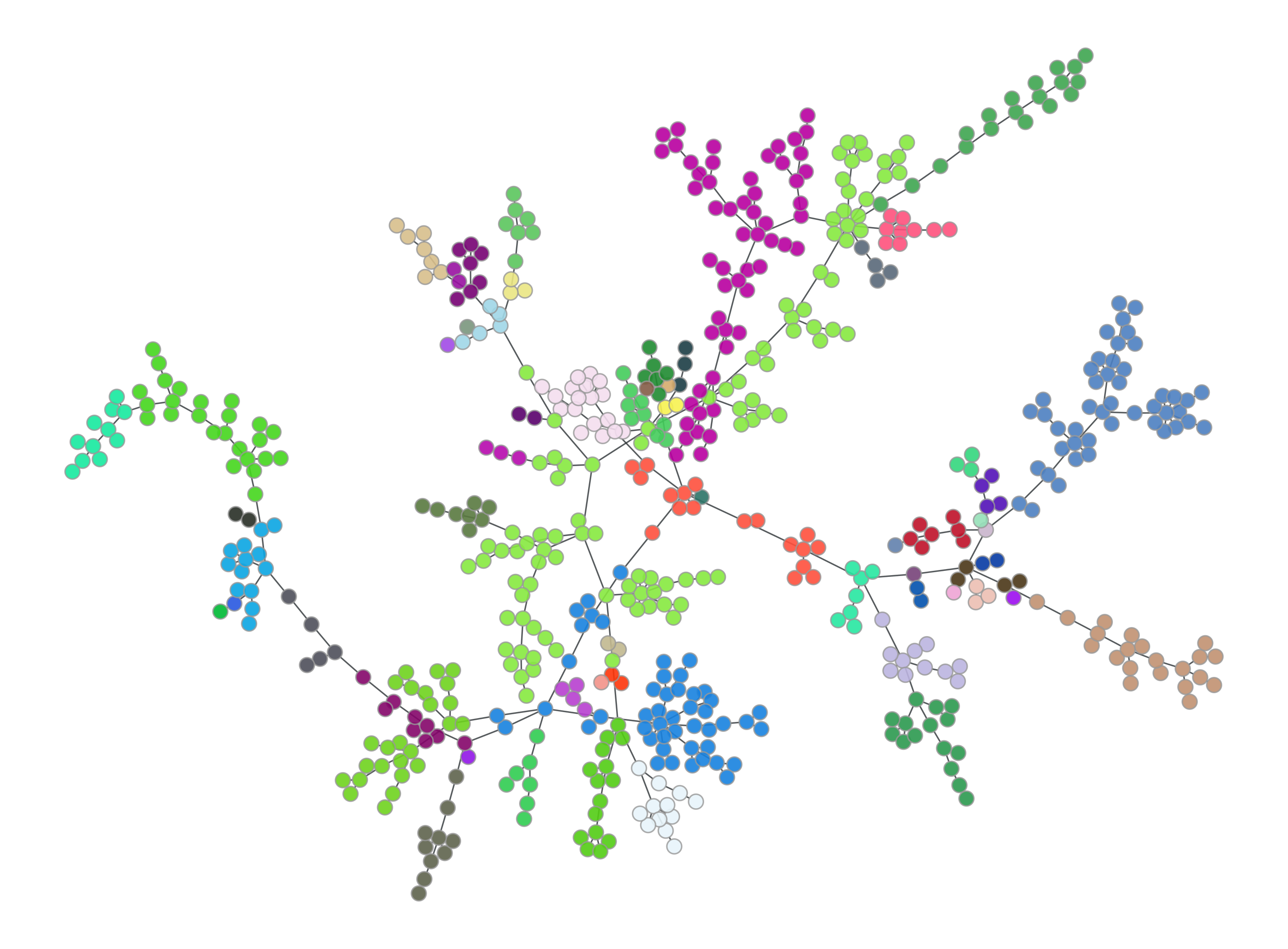
Note that the clusters produced from your high rank fit are likely to be meaningless, so use clusters
from a fit you are happy with. These are combined to give samples coloured by strain in the first plot:

With big data#
For very large datasets, producing a dense distance matrix at all may become totally
infeasible. Fortunately, it is possible to add to the sparse matrix iteratively by making
a lineage fit to a subset of your data, and then repeatedly adding in blocks with poppunk_assign
and --update-db:
poppunk --create-db --r-files qfile1.txt --output listeria_1
poppunk --fit-model lineage --ref-db listeria_1 --ranks 500 --threads 16
poppunk_assign --ref-db listeria_1 --q-files qfile2.txt --output listeria_1 --threads 16 --update-db
poppunk_assign --ref-db listeria_1 --q-files qfile3.txt --output listeria_1 --threads 16 --update-db
This will calculate all vs. all distances, but many of them will be discarded at each stage, controlling the total memory required. The manner in which the sparse matrix grows is predictable: \(Nk + 2NQ + Q^2 - Q\) distances are saved at each step, where \(N\) is the number of references, \(Q\) is the number of requires queries and \(k\) is the rank.
If you split the samples into roughly equally sized blocks of \(Q\) samples, the \(Q^2\) terms dominate. So you can pick \(Q\) such that \(\sim3Q^2\) distances can be stored (each distance uses four bytes). The final distance matrix will contain \(Nk\) distances, so you can choose a rank such that this will fit in memory.
You may then follow the process described above to use poppunk_visualise to generate an MST
from your .npz file after updating the database multiple times.
Using GPU acceleration for the graph#
As an extra optimisation, you may add --gpu-graph to use cuGraph
from the RAPIDS library to calculate the MST on a GPU:
poppunk_visualise --ref-db listeria --tree both --rank-fit sparse_mst/sparse_mst_rank50_fit.npz\
--microreact --output sparse_mst_viz --threads 4 --gpu-graph

Graph-tools OpenMP parallelisation enabled: with 1 threads
Loading distances into graph
Calculating MST (GPU part)
Label prop iterations: 6
Label prop iterations: 5
Label prop iterations: 5
Label prop iterations: 4
Label prop iterations: 2
Iterations: 5
12453,65,126,13,283,660
Calculating MST (CPU part)
Completed calculation of minimum-spanning tree
Generating output
Drawing MST
This uses cuDF to load the sparse matrix (network edges) into the device, and cuGraph to do the MST calculation. At the end, this is converted back into graph-tool format for drawing and output. Note that this process incurs some overhead, so will likely only be faster for very large graphs where calculating the MST on a CPU is slow.
To turn off the graph layout and drawing for massive networks, you can use --no-plot.
Important
The RAPIDS packages are not included in the default PopPUNK installation, as they are in non-standard conda channels. To install these packages, see the guide.